Using Histograms and Descriptive Statistics to Investigate Process Data

A simple summary of descriptive statistics is often the first step in investigating what the data have to say about the process being studied during process improvement initiatives. Questions like “Where is the central tendency?” and “Is this a skewed process?” can quickly be answered by the visual representation that a histogram provides (shape, central tendency, spread, skewness, and normality) alongside statistics derived from the observed data. Let’s have a look at one example using our preferred package SigmaXL©.

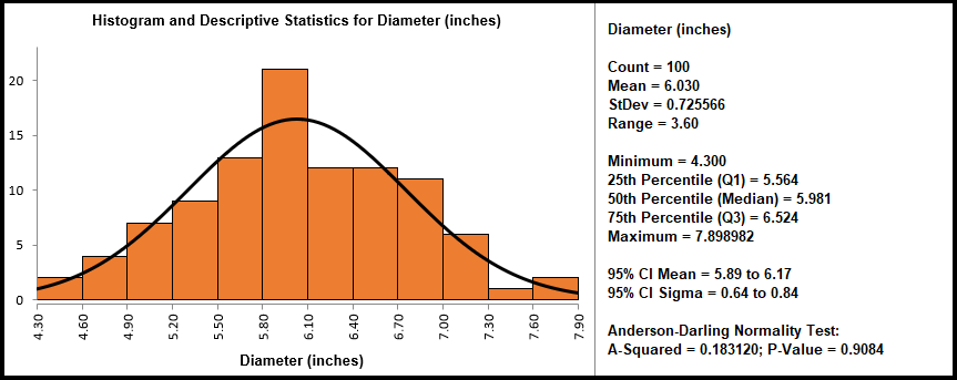
A manufacturing process produces a part that is measured in inches (the same analysis and statistics could also be used in transactional processes such as waiting time in a call center or how many people go through security at an airport). The image above is the histogram for this process along with its descriptive statistics.
- The histogram showcases a bell-shaped distribution: the data seem to be normally distributed. This is confirmed by the P-value for the Anderson-Darling normality test, which in this case, is far greater than an assumed alpha risk of 0.05 (or 5%). In this case, our P-value has a strong case in favour of the Null Hypothesis – which states that there is no difference between this dataset and a normally distributed dataset.
- Starting at the top of the summary box, a simple run of the key statistics: Count (how many data points), Mean (or average), Stdev (for standard deviation) and Range (another measurement of spread)
- The mid-section of the statistics showcases the 5-number summary. Here we can learn about where the data fall in terms of quartiles. Notice that 25% of the data fall under 5.564 inches, the median point is 5.981 inches (50th percentile), and 75% of the data fall under 6.524 inches.
- Finally, we can estimate the true population mean and standard deviation by looking at the Confidence Intervals (CI) built for this specific dataset.
In summary, running histograms and descriptive statistics such as these will quickly provide the analyst with important information about the process data under investigation.

